18. Backpropagation Through Time (part b)
We will now unfold the model. You will see that unfolding the model in time is very helpful in visualizing the number of steps (translated into multiplication) needed in the Backpropagation Through Time process. These multiplications stem from the chain rule and are easily visualized using this model.
In this video we will understand how to use Backpropagation Through Time (BPTT) when adjusting two weight matrices:
- W_y - the weight matrix connecting the state the output
- W_s - the weight matrix connecting one state to the next state
20 RNN BPTT B V5 Final
The unfolded model can be very helpful in visualizing the BPTT process.
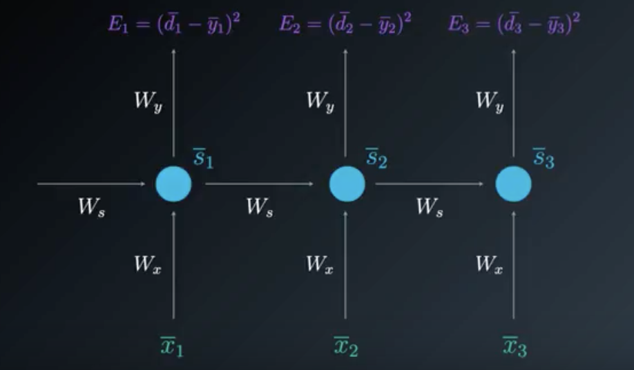
The Unfolded Model at timestep 3
Gradient calculations needed to adjust W_y
The partial derivative of the Loss Function with respect to W_y is found by a simple one step chain rule:
(Note that in this case we do not need to use BPTT. Visualization of the calculations path can be found in the video).
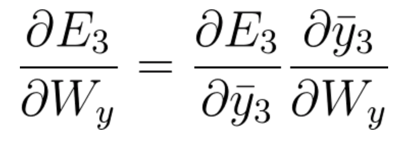
Equation 36
Generally speaking, we can consider multiple timesteps back, and not only 3 as in this example. For an arbitrary timestep N, the gradient calculation needed for adjusting W_y, is:
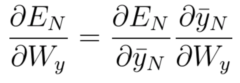
Equation 37
Gradient calculations needed to adjust W_s
We still need to adjust W_s the weight matrix connecting one state to the next and W_x the weight matrix connecting the input to the state. We will arbitrarily start with W_s.
To understand the BPTT process, we can simplify the unfolded model. We will focus on the contributions of W_s to the output, the following way:
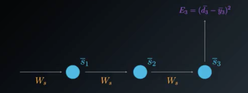
Simplified Unfolded model for Adjusting Ws
When calculating the partial derivative of the Loss Function with respect to W_s, we need to consider all of the states contributing to the output. In the case of this example it will be states \bar{s_3} which depends on its predecessor \bar{s_2} which depends on its predecessor \bar{s_1}, the first state.
In BPTT we will take into account every gradient stemming from each state, accumulating all of these contributions.
- At timestep t=3, the contribution to the gradient stemming from \bar{s_3} is the following :
(Notice the use of the chain rule here. If you need, go back to the video to visualize the calculation path).

Equation 38
- At timestep t=3, the contribution to the gradient stemming from \bar{s_2} is the following :
(Notice how the equation, derived by the chain rule, considers the contribution of \bar{s_2} to \bar{s_3} . If you need, go back to the video to visualize the calculation path).

Equation 39
- At timestep t=3, the contribution to the gradient stemming from \bar{s_1} is the following :
(Notice how the equation, derived by the chain rule, considers the contribution of \bar{s_1} to \bar{s_2} and \bar{s_3} . If you need, go back to the video to visualize the calculation path).

Equation 40
After considering the contributions from all three states: \bar{s_3} ,\bar{s_2} and \bar{s_1}, we will accumulate them to find the final gradient calculation.
The following equation is the gradient contributing to the adjustment of W_s using Backpropagation Through Time:
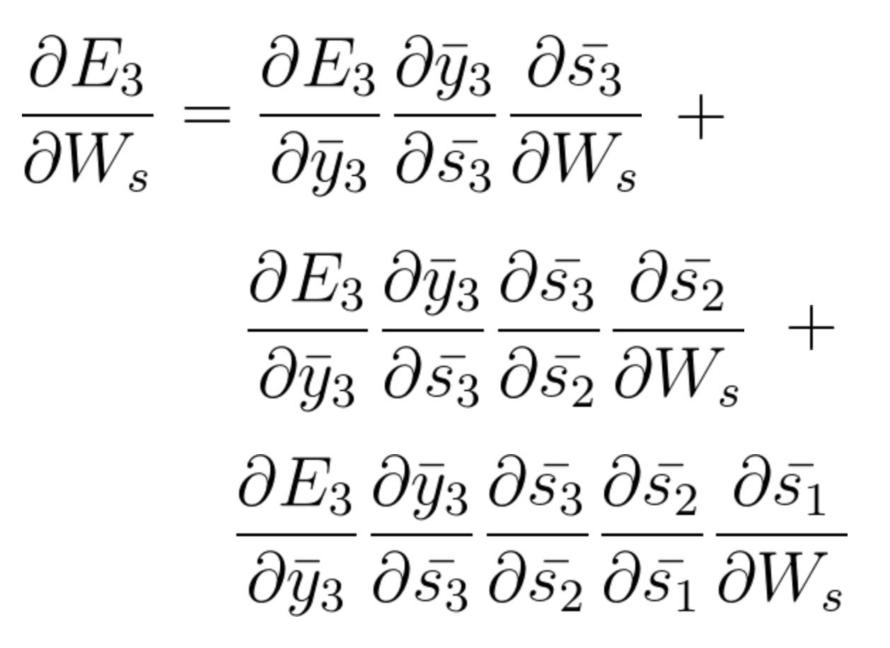
Equation 41
In this example we had 3 time steps to consider, therefore we accumulated three partial derivative calculations. Generally speaking, we can consider multiple timesteps back. If you look closely at the three components of equation 41, you will notice a pattern. You will find that as we propagate a step back, we have an additional partial derivatives to consider in the chain rule. Mathematically this can be easily written in the following general equation for adjusting W_s using BPTT:

Equation 42
Notice that Equation 6 considers a general setting of N steps back. As mentioned in this lesson, capturing relationships that span more than 8 to 10 steps back is practically impossible due to the vanishing gradient problem. We will talk about a solution to this problem in our LSTM section coming up soon.
We still need to adjust W_x, the weight matrix connecting the input to the state.
Let's take a small break. You can use this time to go over the BPTT process we've seen so far. Try to get yourself comfortable with the math.
Once you are feeling confident with the content of the video you just viewed, try to derive the calculations for adjusting the last matrix, W_x by yourself. This is by no means a must, but if you feel that you are up for the challenge, go for it! It will be interesting to compare your notes with ours.
If you chose to take on the challenge, focus on simplifying the unfolded model, leaving only what you need for the calculations. Sketch the backpropagation "path", and step by step think of how the chain rule helps with the derivations here. Don't forget to** accumulate!**.